|
In Issue 4's coverage of Kernel Density Estimation (KDE) we explored how one can estimate the underlying source probability density function (PDF) given only a finite number of random samples from that distribution. Now, we explore the reverse problem: how do we generate random samples from a given PDF target? The data we have been working with throughout this newsletter have all been synthetic (computer-generated) and many programs use this method of Markov Chain Monte Carlo (MCMC) under-the-hood. In fact, a lot of research in modern statistics has gone towards developing more efficient techniques of "probabilistic programming," as MCMC has a vast array of applications, from protein folding and drug simulations to financial and weather modeling.
|
Random Walk Metropolis
Let's try and formalize our goal a bit more concretely. We want to generate pseudorandom numbers ("pseudo" because we have some control over how they are being generated), such that, when taken together, the sequence of pseudorandom numbers we generate follows the same distribution as the target PDF. Consider the following "random walk Metropolis" algorithm for generating a random walk on the real numbers. The Metropolis algorithm (a special case of the more general "Metropolis–Hastings algorithm") is especially noteable because it is easy to explain, has an appealing, intuitive idea, and can be used in a great variety of ways.
Algorithm 1 Metropolis algorithm
Choose a target PDF p and a proposal distribution q for possible candidates
Choose an initial sample
for do
end for
Essentially, we propose a "candidate" point to move to, chosen by drawing from some other distribution we're already able to sample from. Then we make a probabilistic decision of whether or not to "accept" and move to the location of the candidate. If the candidate is in a region of higher probability we will always accept. However, even if the candidate is in a region of lower probability, we instead accept it with probability of the ratio between the PDF(candidate) / PDF(current). This probabilistic acceptance of candidates in regions of lower probability density, results in a random walk that doesn't get stuck in regions of high probability density, but rather, spends time proportional to the target PDF.
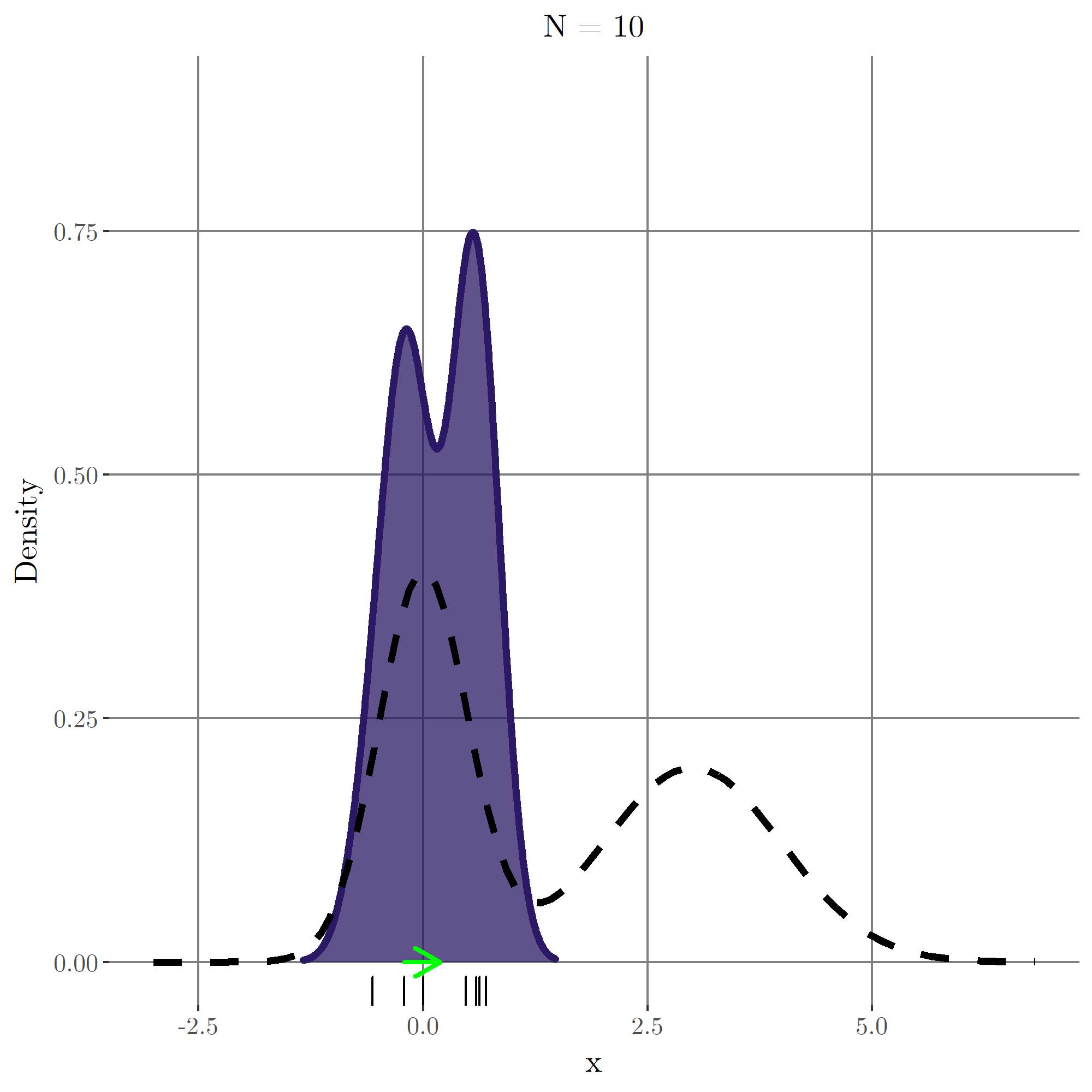
This process is visualized in the simulation above. The dashed black line is the desired target PDF, according to which we wish to generate samples. The colorfully shaded curve is running the KDE of our N samples so far. The black tickmarks below the graph are the points we've visited/samples we've generated. The green arrow is a candidate that was accepted; the red arrow is a candidate that was rejected. We see that as the number N of samples grows large, we get a random walk whose states are distributed according to the target PDF, as desired.
|